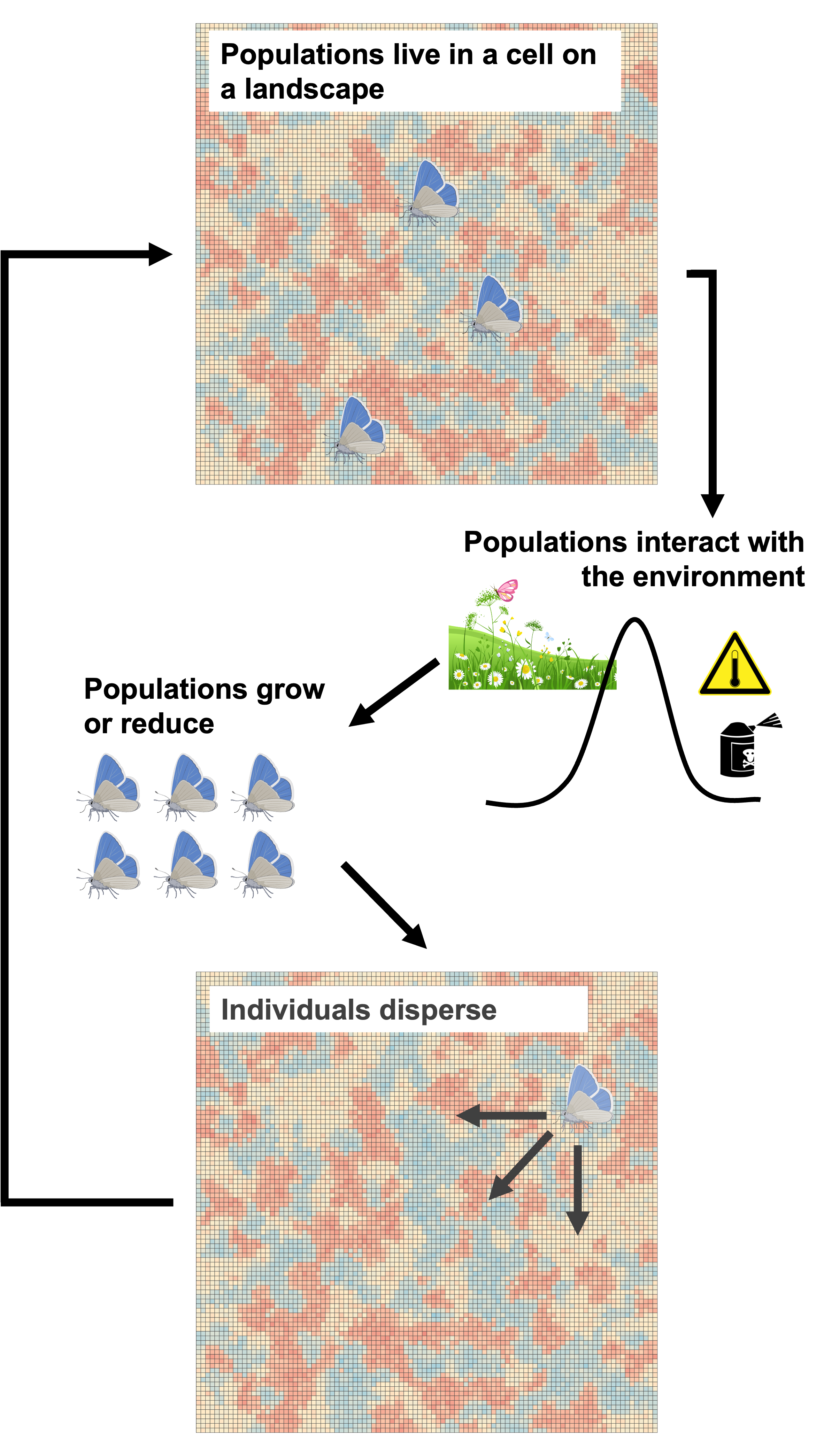
Simulation
Before pressing go
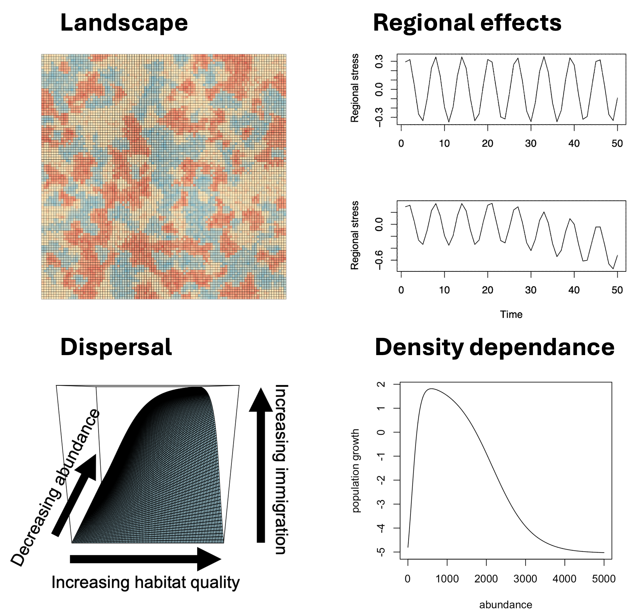
Landscapes
Descriptions of landscape generation can be found on the landscapes page. Landscapes vary in the proportion of land types, the patchiness of the landscape, and the strength of additional localized stressors.
Regional effects
We simulate effects that impact the entire landscape, regardless of land use type. This is meant to simulate large climate phenomena like El Niño cycles and large-scale climate change. In a no-trend scenario, there are oscillations of good years and bad years, and imposing a trend makes bad years more frequent.
Density dependence
We impose density-dependent effects on each cell in the simulation, where high and low numbers of individuals are associated with negative population growth.
Dispersal
Dispersal is programmed using two parameters. The first determines how far a species can disperse in a single time step. Within this range, the probability is inverse to the distance from the reference cell. We also added a component of choice, where individuals prefer to go to locations of higher quality habitat with fewer individuals. The second parameter determines the propensity to disperse for a particular species. A wide-ranging species will have access to more cells each time step and will see more individuals leave due to dispersal. This second parameter also is the scaler for the first. If 50% of individuals will leave a cell, it is this 50% that are moved throughout the landscape inversely proportionally to distance.